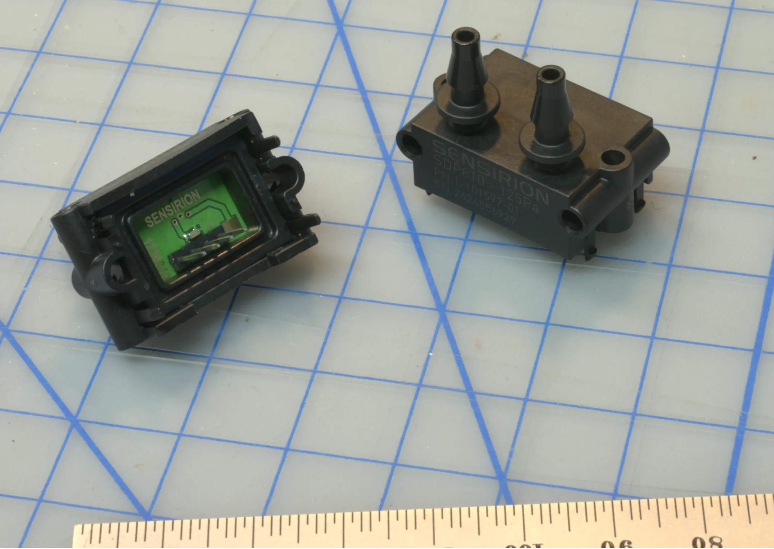
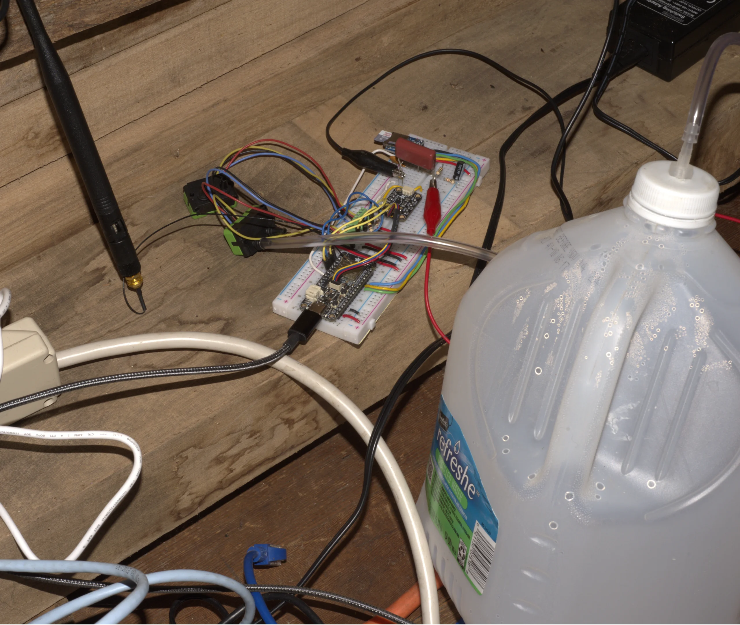
Confirmed: Milk Jug Transducer Captures Train Infrasounds

<p>Today is a milestone for I have proven that a $35 Sensirion <a title="https://www.digikey.com/en/products/detail/sensirion-ag/SDP810-125PA/6605488?s=N4IgTCBcDaIMoBEAKAOAjABgLRrAViQEMQBdAXyA" href="https://www.digikey.com/en/products/detail/sensirion-ag/SDP810-125PA/6605488?s=N4IgTCBcDaIMoBEAKAOAjABgLRrAViQEMQBdAXyA" data-from-md="">SDP810-125PA</a> differential pressure transducer, connected to an ordinary empty milk jug, detected low-frequency pressure fluctuations coinciding with a freight train passing approximately 1,300 feet away.This physical setup of using back pressure on a transducer is based on the article by Marcello <em>et al.</em> “Implementation, Characterization, and Evaluation of an Inexpensive Low-Power Low-Noise Infrasound Sensor Based on a Micromachined Differential Pressure Transducer and a Mechanical Filter” (2012). 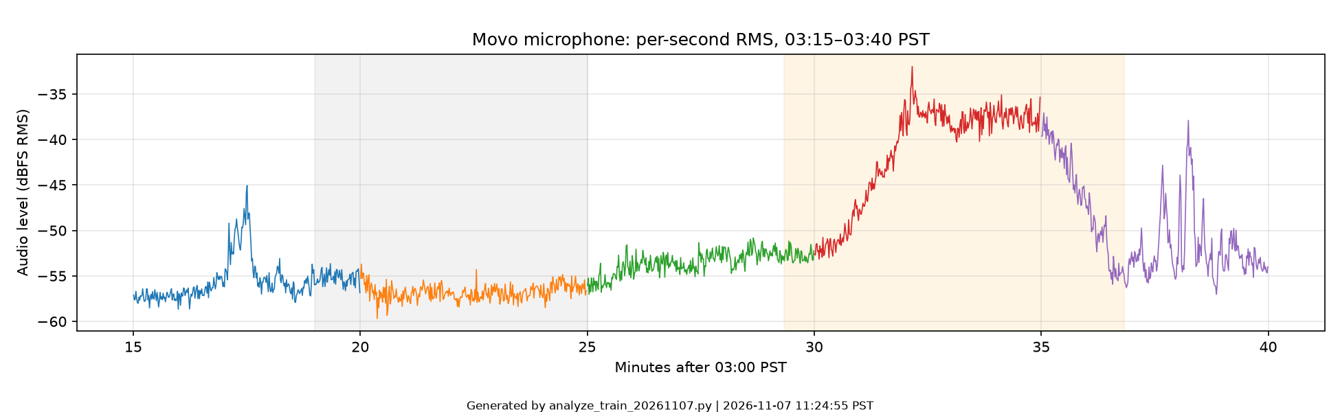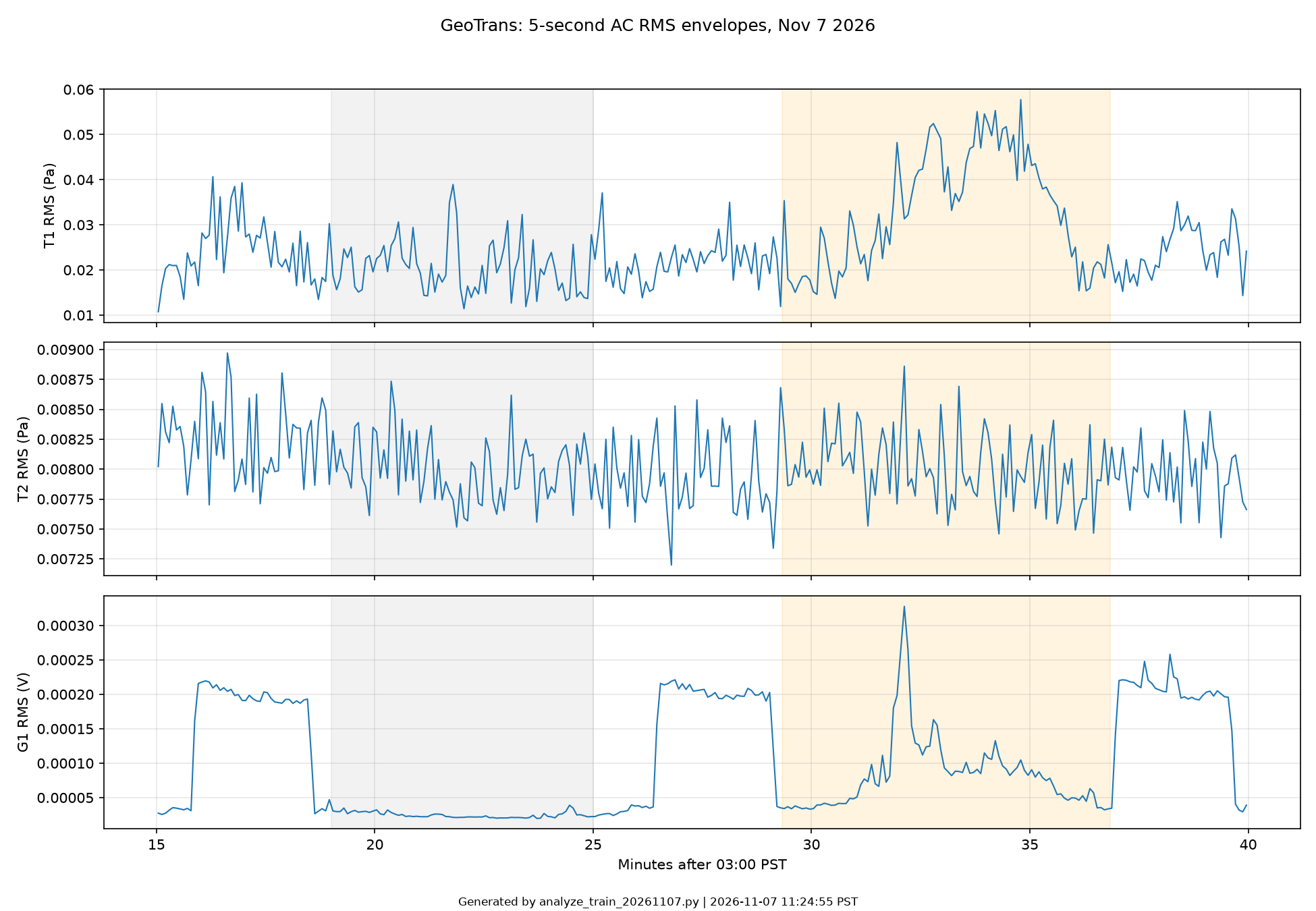(See note below.)</p> <img class=" wp-image-1338" src="https://salemdata.net/johnpress/wp-content/uploads/2026/11/DSC_5698-scaled.webp" alt="" width="646" height="545" /> Circuit breadboard in a nest of wires with milk jug <p>A freight train came by at 3:30 AM, Saturday morning, November 7, 2026. At that time I was logging audio (44,000 Hz) with a microphone outdoors and indoors two transducers (air pressure) at 100 readings/second each, and one geophone vertical seismic motion at 330 readings/second. Here are the analyses.</p> <h2>Audio recording</h2> <p>The gray area is a quiet period, the tan area is during the train event. These two areas were arbitrarily defined by me to have two “envelopes”: one of quiet and the other during the train event.</p> <img class=" wp-image-1339" src="https://salemdata.net/johnpress/wp-content/uploads/2026/11/05_audio_rms.png" alt="" width="540" height="166" /> Audio 11/7/26 <p>Sensor Recording</p> <p>Here are the three sensors. T2 is the “control” transducer which has both port open. T1 is the transducer that has one port connected to a leading milk jug to provide back pressure. 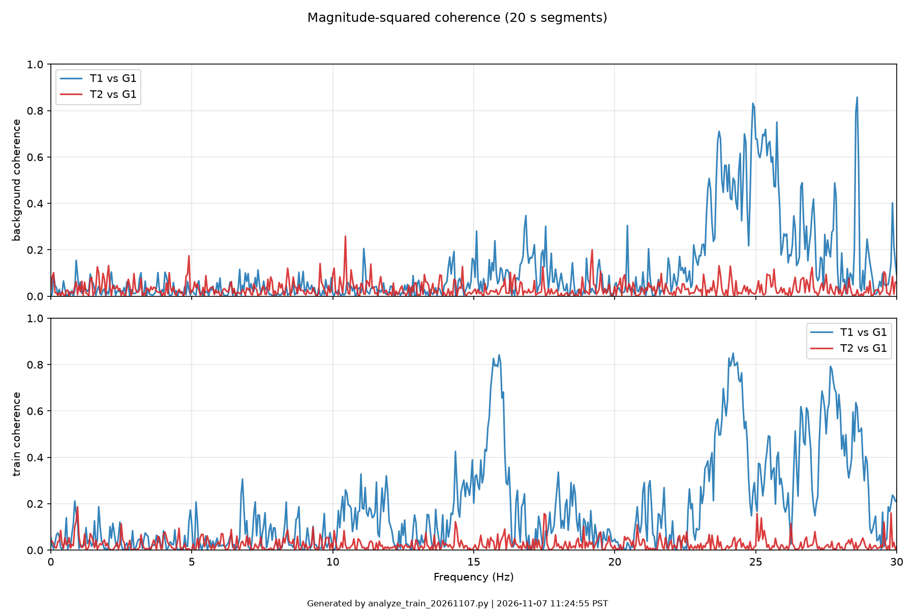The gray and tan time lines previously described are overlayed here.</p> <p><img class=" wp-image-1341 aligncenter" src="https://salemdata.net/johnpress/wp-content/uploads/2026/11/01_signal_envelopes.png" alt="" width="430" height="297" /></p> <h2>Magnitude-squared</h2> <p>This graph compares the readings from the two pressure sensors (T1 and T2) with the geophone (G1), which measures ground vibrations. The higher the line, the more closely the two instruments’ readings are related at that frequency. A value of 1 indicates a very strong relationship; a value of 0 indicates no consistent relationship.</p> <p>The blue line represents the milk-jug sensor (T1), while the red line represents the control sensor (T2), which has both ports open. Notice how the blue line rises at certain frequencies while the red line remains relatively low. 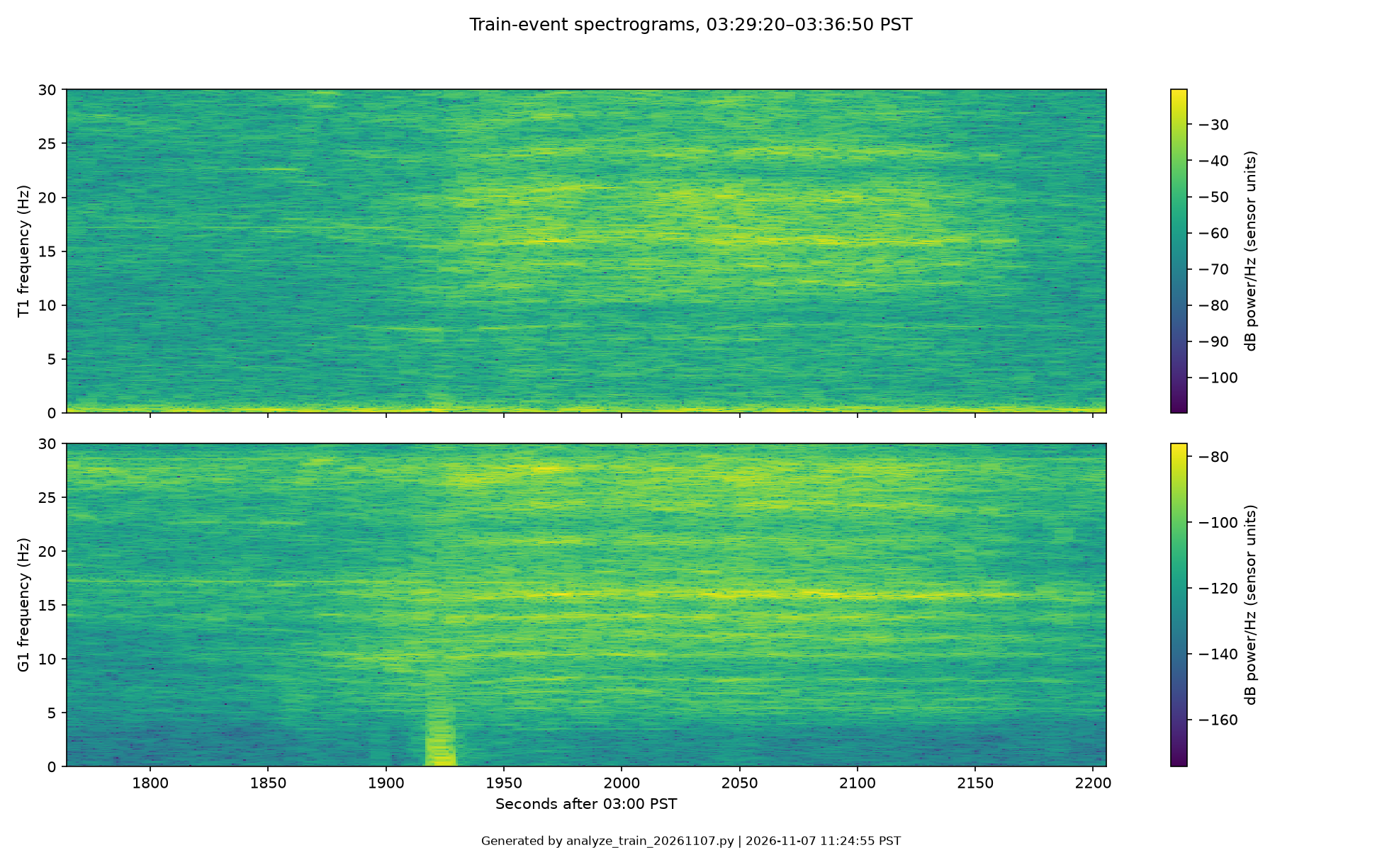This indicates that the milk-jug sensor detected patterns corresponding to the ground vibrations that the control sensor did not.</p> <img class=" wp-image-1340" src="https://salemdata.net/johnpress/wp-content/uploads/2026/11/04_coherence.png" alt="" width="507" height="338" /> Transducers and geophone values <h2>Spectrogram</h2> <p>This spectrogram is for the train event only and for the T1 milk jug transducer and the geophone (“G1”).</p> <p><img class=" wp-image-1342 aligncenter" src="https://salemdata.net/johnpress/wp-content/uploads/2026/11/03_train_spectrograms.png" alt="" width="387" height="238" /></p> <h2>Frequency Analysis</h2> <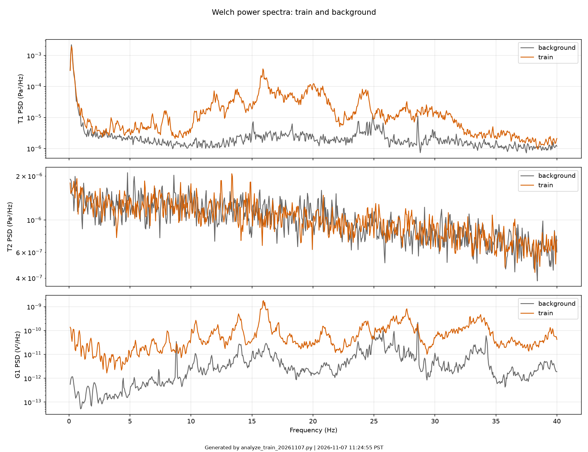p>This is the most important chart: it shows frequencies that were captured both during the quiet event and the train event. You can see, for example, in the T1 comparison just above 15 Hz there is a noticeable peak when compared to the control. T2 shows that nothing was measured by the T2 transducer during the train event when compared with the quiet event. And the geophone shows it detected an increase of frequencies during the train event.</p> <img class=" wp-image-1343" src="https://salemdata.net/johnpress/wp-content/uploads/2026/11/02_welch_psd.png" alt="" width="617" height="474" /> Frequency Analysis <h2 role="listitem">Conclusion</h2> <p>During the freight train event, there were low frequencies detected by T1 when compared with a quiet period just minutes before. The back-pressured transducer detected pressure differences during a train event. Hence, addition of a back-pressure to the transducer allows it to detect low frequencies.</p> <p>While the Marcillo back-pressure is carefully devised and tested, mine was just a simple: does it work rough test against a train event. I know from previous tests that low level seismic frequencies are present when freight trains come by, these results demonstrate that low level audio frequencies, ie. through the air as compared with seismic “through the ground”, occur during train events. I will now refine the physical back-pressure mechanism and test.</p> <h6>Note:</h6> <div id="refs" class="references csl-bib-body hanging-indent" role="list"> <div id="ref-ImplementationCharacterizationandEvaluationofanInexpensiveLowPowerLowNoiseInfrasoundSensorBasedonaMicromachinedDifferentialPressureTransducerandaMechanicalFilter" class="csl-entry" role="listitem">Marcillo, Omar, Jeffrey B. Johnson, and Darren Hart. 2012.<br /> “Implementation, Characterization, and Evaluation of an<br /> Inexpensive Low-Power Low-Noise Infrasound Sensor Based on a<br /> Micromachined Differential Pressure Transducer and a Mechanical<br /> Filter.” <em>Journal of Atmospheric and Oceanic Technology</em><br /> (Boston MA, USA) 29 (9): 1275-84. <a href="https://doi.org/10.1175/JTECH-D-11-00101.1">https://doi.org/10.1175/JTECH-D-11-00101.1</a>.</div> </div> <p>Here is a summary:</p> <pre>Analysis script: analyze_train_20261107.py Run: 2026-11-07 11:24:55 PST Input log: geotrans_20261107_Sat_030000.log Audio: saturday_train.zip Train: 03:29:20–03:36:50 PST; Background 03:19:00–03:25:00 PST T1 background detrended RMS: 0.024355207; top PSD peaks: [0.2, 0.65, 0.9, 24.9, 28.6, 23.75, 15.1, 24.65] train detrended RMS: 0.04075246; top PSD peaks: [0.2, 15.9, 15.75, 16.2, 16.05, 20.05, 19.8, 19.6] Band (0.1, 1): train 0.000342685, bg 0.000360437, ratio -0.22 dB Band (1, 5): train 2.04647e-05, bg 1.11463e-05, ratio 2.64 dB Band (5, 20): train 0.000537886, bg 3.02347e-05, ratio 12.50 dB Band (20, 40): train 0.000293156, bg 3.93389e-05, ratio 8.72 dB T2 background detrended RMS: 0.0068583718; top PSD peaks: [4.8, 8.6, 0.5, 5.35, 1.2, 9.8, 7.65, 0.65] train detrended RMS: 0.006869717; top PSD peaks: [13.35, 0.65, 12.5, 6.2, 0.4, 14.9, 9.15, 10.0] Band (0.1, 1): train 1.34688e-06, bg 1.28021e-06, ratio 0.22 dB Band (1, 5): train 5.04324e-06, bg 5.05579e-06, ratio -0.01 dB Band (5, 20): train 1.77835e-05, bg 1.78006e-05, ratio -0.00 dB Band (20, 40): train 1.64998e-05, bg 1.61447e-05, ratio 0.09 dB G1 background detrended RMS: 2.2681042e-05; top PSD peaks: [28.6, 25.75, 26.65, 25.45, 34.2, 24.9, 25.05, 25.25] train detrended RMS: 8.6053226e-05; top PSD peaks: [15.95, 16.05, 27.7, 15.7, 16.3, 13.9, 33.75, 26.85] Band (0.1, 1): train 5.14341e-11, bg 4.02122e-13, ratio 21.07 dB Band (1, 5): train 4.28721e-11, bg 9.20576e-13, ratio 16.68 dB Band (5, 20): train 1.56285e-09, bg 6.73316e-11, ratio 13.66 dB Band (20, 40): train 2.09853e-09, bg 2.00237e-10, ratio 10.20 dB Coherence background T1 vs G1: top frequencies [(16.85, 0.348), (17.55, 0.301), (16.8, 0.295), (15.1, 0.281), (15.75, 0.239), (17.15, 0.222), (11.1, 0.206), (16.9, 0.202), (17.45, 0.198), (14.3, 0.193)] T2 vs G1: top frequencies [(10.45, 0.259), (19.2, 0.2), (4.9, 0.174), (9.55, 0.141), (11.35, 0.138), (2.05, 0.132), (19.15, 0.129), (14.6, 0.128), (17.45, 0.127), (1.65, 0.127)] Coherence train T1 vs G1: top frequencies [(15.9, 0.842), (15.7, 0.826), (15.95, 0.81), (15.8, 0.799), (15.75, 0.794), (15.85, 0.791), (15.65, 0.76), (15.6, 0.696), (16.05, 0.682), (16.0, 0.656)] T2 vs G1: top frequencies [(0.95, 0.187), (17.5, 0.158), (17.55, 0.152), (0.9, 0.124), (14.35, 0.123), (2.5, 0.114), (0.85, 0.103), (18.9, 0.102), (9.3, 0.098), (4.55, 0.095)] Generated by analyze_train_20261107.py | 2026-11-07 11:24:55 PST </pre>

Today is a milestone for I have proven that a $35 Sensirion SDP810-125PA differential pressure transducer, connected to an ordinary empty milk jug, detected low-frequency pressure fluctuations coinciding with a freight train passing approximately 1,300 feet away.This physical setup of using back pressure on a transducer is based on the article by Marcello et al. “Implementation, Characterization, and Evaluation of an Inexpensive Low-Power Low-Noise Infrasound Sensor Based on a Micromachined Differential Pressure Transducer and a Mechanical Filter” (2012). (See note below.)

Circuit breadboard in a nest of wires with milk jug

A freight train came by at 3:30 AM, Saturday morning, November 7, 2026. At that time I was logging audio (44,000 Hz) with a microphone outdoors and indoors two transducers (air pressure) at 100 readings/second each, and one geophone vertical seismic motion at 330 readings/second. Here are the analyses.

Audio recording

The gray area is a quiet period, the tan area is during the train event. These two areas were arbitrarily defined by me to have two “envelopes”: one of quiet and the other during the train event.

Sensor Recording

Here are the three sensors. T2 is the “control” transducer which has both port open. T1 is the transducer that has one port connected to a leading milk jug to provide back pressure. The gray and tan time lines previously described are overlayed here.

Magnitude-squared

This graph compares the readings from the two pressure sensors (T1 and T2) with the geophone (G1), which measures ground vibrations. The higher the line, the more closely the two instruments’ readings are related at that frequency. A value of 1 indicates a very strong relationship; a value of 0 indicates no consistent relationship.

The blue line represents the milk-jug sensor (T1), while the red line represents the control sensor (T2), which has both ports open. Notice how the blue line rises at certain frequencies while the red line remains relatively low. This indicates that the milk-jug sensor detected patterns corresponding to the ground vibrations that the control sensor did not.

Spectrogram

This spectrogram is for the train event only and for the T1 milk jug transducer and the geophone (“G1”).

Frequency Analysis

This is the most important chart: it shows frequencies that were captured both during the quiet event and the train event. You can see, for example, in the T1 comparison just above 15 Hz there is a noticeable peak when compared to the control. T2 shows that nothing was measured by the T2 transducer during the train event when compared with the quiet event. And the geophone shows it detected an increase of frequencies during the train event.

Conclusion

During the freight train event, there were low frequencies detected by T1 when compared with a quiet period just minutes before. The back-pressured transducer detected pressure differences during a train event. Hence, addition of a back-pressure to the transducer allows it to detect low frequencies.

While the Marcillo back-pressure is carefully devised and tested, mine was just a simple: does it work rough test against a train event. I know from previous tests that low level seismic frequencies are present when freight trains come by, these results demonstrate that low level audio frequencies, ie. through the air as compared with seismic “through the ground”, occur during train events. I will now refine the physical back-pressure mechanism and test.

Note:

Marcillo, Omar, Jeffrey B. Johnson, and Darren Hart. 2012.
“Implementation, Characterization, and Evaluation of an
Inexpensive Low-Power Low-Noise Infrasound Sensor Based on a
Micromachined Differential Pressure Transducer and a Mechanical
Filter.” Journal of Atmospheric and Oceanic Technology
(Boston MA, USA) 29 (9): 1275-84. https://doi.org/10.1175/JTECH-D-11-00101.1.

Here is a summary:

Analysis script: analyze_train_20261107.py
Run: 2026-11-07 11:24:55 PST
Input log: geotrans_20261107_Sat_030000.log
Audio: saturday_train.zip
Train: 03:29:20–03:36:50 PST; Background 03:19:00–03:25:00 PST

T1
 background detrended RMS: 0.024355207; top PSD peaks: [0.2, 0.65, 0.9, 24.9, 28.6, 23.75, 15.1, 24.65]
 train detrended RMS: 0.04075246; top PSD peaks: [0.2, 15.9, 15.75, 16.2, 16.05, 20.05, 19.8, 19.6]
 Band (0.1, 1): train 0.000342685, bg 0.000360437, ratio -0.22 dB
 Band (1, 5): train 2.04647e-05, bg 1.11463e-05, ratio 2.64 dB
 Band (5, 20): train 0.000537886, bg 3.02347e-05, ratio 12.50 dB
 Band (20, 40): train 0.000293156, bg 3.93389e-05, ratio 8.72 dB

T2
 background detrended RMS: 0.0068583718; top PSD peaks: [4.8, 8.6, 0.5, 5.35, 1.2, 9.8, 7.65, 0.65]
 train detrended RMS: 0.006869717; top PSD peaks: [13.35, 0.65, 12.5, 6.2, 0.4, 14.9, 9.15, 10.0]
 Band (0.1, 1): train 1.34688e-06, bg 1.28021e-06, ratio 0.22 dB
 Band (1, 5): train 5.04324e-06, bg 5.05579e-06, ratio -0.01 dB
 Band (5, 20): train 1.77835e-05, bg 1.78006e-05, ratio -0.00 dB
 Band (20, 40): train 1.64998e-05, bg 1.61447e-05, ratio 0.09 dB

G1
 background detrended RMS: 2.2681042e-05; top PSD peaks: [28.6, 25.75, 26.65, 25.45, 34.2, 24.9, 25.05, 25.25]
 train detrended RMS: 8.6053226e-05; top PSD peaks: [15.95, 16.05, 27.7, 15.7, 16.3, 13.9, 33.75, 26.85]
 Band (0.1, 1): train 5.14341e-11, bg 4.02122e-13, ratio 21.07 dB
 Band (1, 5): train 4.28721e-11, bg 9.20576e-13, ratio 16.68 dB
 Band (5, 20): train 1.56285e-09, bg 6.73316e-11, ratio 13.66 dB
 Band (20, 40): train 2.09853e-09, bg 2.00237e-10, ratio 10.20 dB

Coherence background
 T1 vs G1: top frequencies [(16.85, 0.348), (17.55, 0.301), (16.8, 0.295), (15.1, 0.281), (15.75, 0.239), (17.15, 0.222), (11.1, 0.206), (16.9, 0.202), (17.45, 0.198), (14.3, 0.193)]
 T2 vs G1: top frequencies [(10.45, 0.259), (19.2, 0.2), (4.9, 0.174), (9.55, 0.141), (11.35, 0.138), (2.05, 0.132), (19.15, 0.129), (14.6, 0.128), (17.45, 0.127), (1.65, 0.127)]

Coherence train
 T1 vs G1: top frequencies [(15.9, 0.842), (15.7, 0.826), (15.95, 0.81), (15.8, 0.799), (15.75, 0.794), (15.85, 0.791), (15.65, 0.76), (15.6, 0.696), (16.05, 0.682), (16.0, 0.656)]
 T2 vs G1: top frequencies [(0.95, 0.187), (17.5, 0.158), (17.55, 0.152), (0.9, 0.124), (14.35, 0.123), (2.5, 0.114), (0.85, 0.103), (18.9, 0.102), (9.3, 0.098), (4.55, 0.095)]

Generated by analyze_train_20261107.py | 2026-11-07 11:24:55 PST