Using Low-Cost GNSS Receivers to Pre-Qualify Survey Sites for NOAA OPUS

Motivation

Most GNSS survey failures are not due to equipment—they are due to poor site selection. Survey-grade GNSS equipment paired with NOAA OPUS processing can achieve centimeter-level accuracy, but deployment is not trivial. Site quality—sky visibility, multipath, and obstruction—directly impacts results.

The central question:

Can low-cost GNSS receivers be used as a reconnaissance tool to determine whether a site is suitable before deploying survey-grade equipment?

Reference Point: Physical Survey Monument

To ground this work in reality, I began with an existing survey control point located adjacent to my property. This provides a known, stable reference—exactly the kind of point that survey-grade workflows rely upon. This point serves as a proxy for a known coordinate, allowing comparison against expected positional stability rather than absolute truth.

Survey control point close-up

Survey control point context

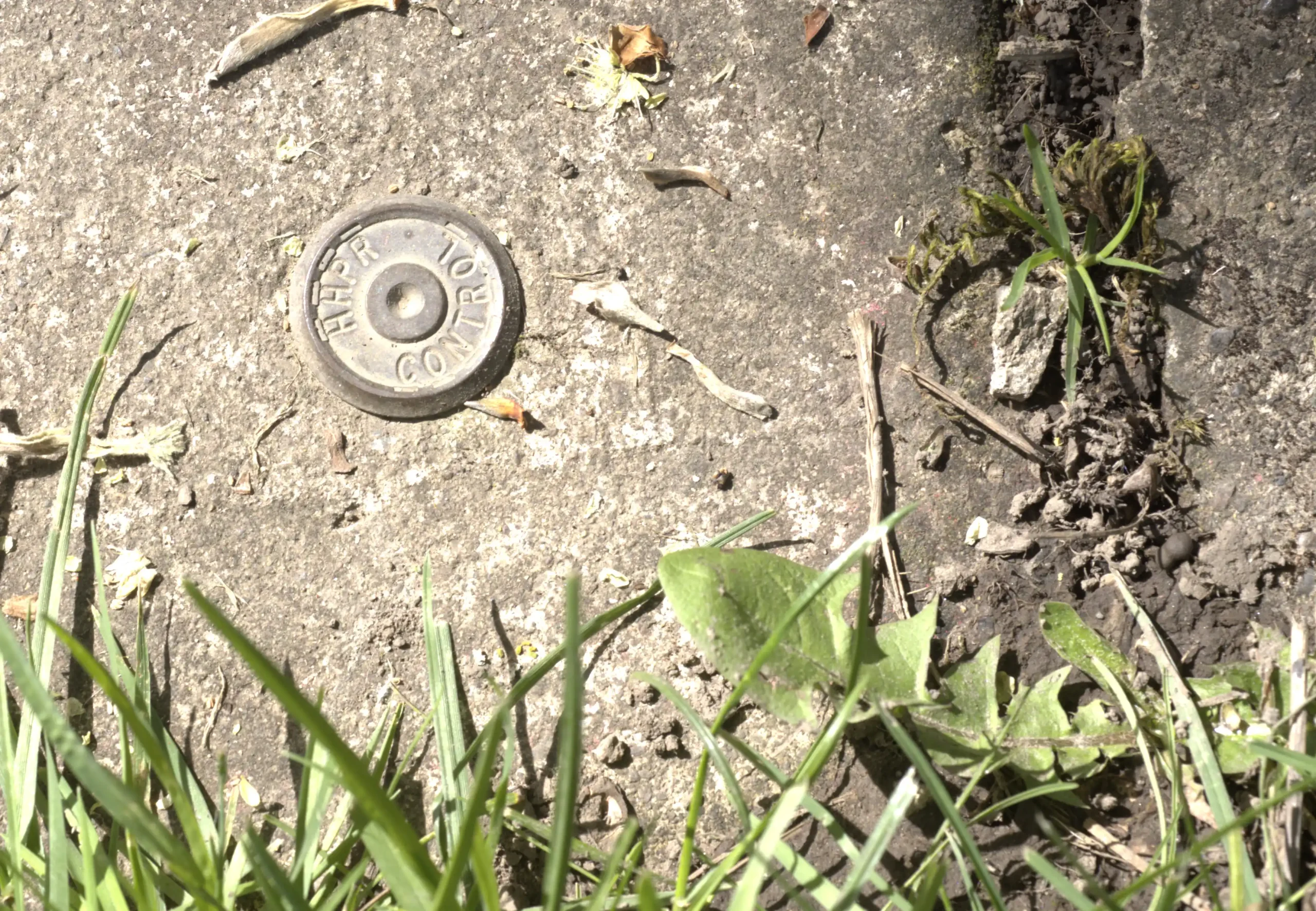
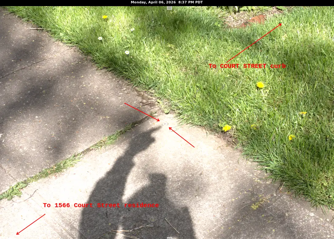
The monument is embedded in the sidewalk and represents a professionally established control point. This allows comparison between low-cost receiver behavior and a location presumed to be well-characterized. Photos taken on Easter Sunday—hunting for survey control points instead of Easter eggs.

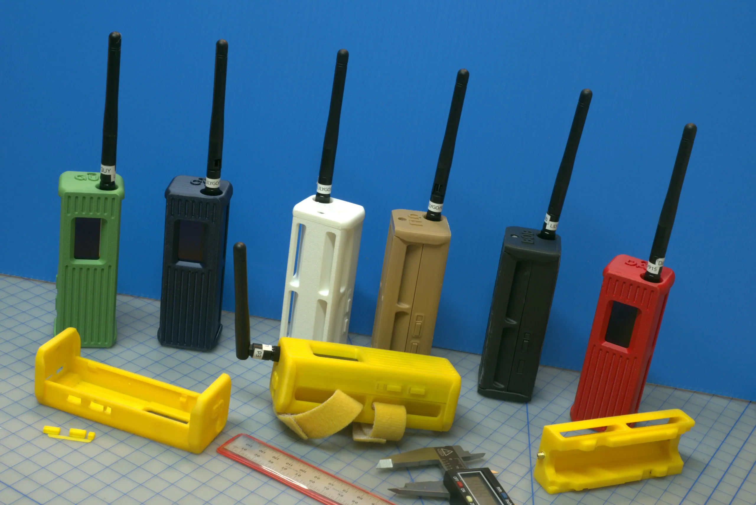
Test Hardware

The data collection platform is based on the LilyGO T-Beam Supreme:

ESP32-S3 platform
GNSS receivers:
- L76K
- u-blox MAX-M10S

Each unit logs raw observational satellite data for later analysis. All receivers were operated concurrently (using GPS time discipline) under identical sky conditions to eliminate temporal variability.

(Yes—there are multiple units, color-coded and named AMY -> GUY. This is deliberate to allow simultaneous multi-receiver comparisons for a study of Reticulum.)

Multi-receiver test set used for simultaneous GNSS logging (color-coded for tracking and analysis)

Data Collection

Typical capture:

Duration: ~30–90 minutes
Samples: 2,000–6,000+ rows per session
Stationary receiver placement

Each record includes:

Satellite count
HDOP
CN0 (signal strength)
Constellation distribution (GPS, GLONASS, etc.)
Computed positional wander

Sampling interval: approximately 1 Hz (varies slightly by receiver).

Analysis Pipeline

Data is ingested into PostgreSQL for analysis.

The workflow:

CSV → PostgreSQL → Aggregation Queries → Comparative Metrics

All metrics are computed over stationary datasets to isolate receiver behavior from movement-induced variance. A sample comparison output is referenced below. Here is the repository for the code (this is an exercise for a tracking project related to Reticulum):

Repository:

https://salemdata.net/repo/jlpoole/microReticulumTbeam/src/branch/feature/fieldtest-beacon-sd-provision/exercises/18_GPS_Field_QA

Example output (excerpt):

avg_sats_used:
  L76K      → 5.29
  MAX-M10S  → 3.70

avg_hdop:
  L76K      → 0.640
  MAX-M10S  → 0.528

avg_cn0:
  L76K      → 31.37
  MAX-M10S  → 24.62

avg_wander_m:
  L76K      → 2.586
  MAX-M10S  → 1.503

Initial Observations

L76K shows higher satellite utilization and stronger signal levels (CN0)
u-blox MAX-M10S exhibits lower positional wander
HDOP differences are modest but measurable

This suggests that different receivers may emphasize different tradeoffs:

Signal richness vs positional stability

The divergence between signal strength (CN0) and positional stability (wander) suggests that receiver filtering and solution algorithms play a significant role beyond raw signal acquisition.

Working Hypothesis

If low-cost receivers consistently exhibit stable geometry (low HDOP), strong signal (high CN0), and low positional dispersion:

Low HDOP
High CN0
Low positional wander

Then the site is likely to perform well under survey-grade GNSS with OPUS processing.

This would allow:

Rapid site screening
Reduced deployment risk
Better placement of high-value equipment

Open Questions

What thresholds meaningfully predict OPUS success?
How strong is correlation between low-cost receivers and survey-grade results?
Are certain constellations (e.g. GLONASS-heavy vs GPS-heavy) more predictive?
How much observation time is “enough”?

Next Steps

Multi-receiver simultaneous logging at multiple sites
Correlation with known control points
Integration with higher-grade GNSS hardware (mosaic-class receivers)

Call for Input

If you are working in:

GNSS / geodesy
RTK / survey workflows
Low-cost GPS experimentation

I would be interested in your observations—especially around thresholds and validation techniques. This work is not intended to replace survey-grade workflows, but to reduce uncertainty prior to deployment.

Sample Output

https://salemdata.us/dev/Satellite_Site_Comparison_2-26-4-6_1955.html